Conditional formatting for multiple columns

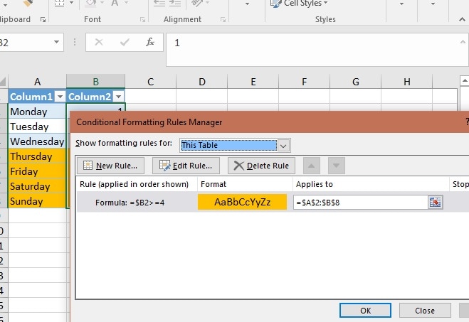
Question: I want to apply conditional formatting to two columns, so that when one column is highlighted by a color, the column next to it is, also.

When I am teaching Excel, the question of how to apply conditional formatting to other columns comes up a lot, and in the past I solved it with a macro or an =if rule mimicking conditional formatting, and this is still a good solution.

However the clever engineer I am married to showed a me a better, more efficient way,  and that is a golden rule: in Excel, efficiency is everything.

To start, I am setting up a simple spreadsheet.  I have the days of the week in Column A1:A7 and numbers 1-7 in Column B1:B7.

For this scenario, I want to say that anything in column B that is greater than 5 is highlighted.  

Step 1: Make your range a table by pressing CRTL+T at the same time.  This inserts a header row, making the table span A1:B8.
Step 2:  Select your cells that should be affected by the conditional formatting.
Step 3: Create a conditional formatting rule.  I will use anything above 4 will be highlighted as yellow.
a. New Rule
b. =$B2>=4 and the formatting is yellow.  Using the $B keeps Excel looking in row B to find a value in 4.  
Step 3: Modify the rules.  This will include column A.  Go  to Modify Rules to open the Conditional Formatting Rules Manager.
a. The rules should apply to =$A$2:$B$8. Use F4 to get the magical $ to indicate absolute value. 
​