If you are new to Excel or you want to work more efficiently, try these tips for using Autosum.Let's start with some basics. If you just want a quick view of a running total, select the numbers and look in the bottom right corner of your screen. 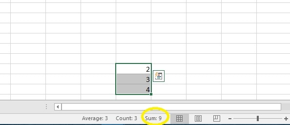 For numbers that will stay in place, you can: Use the Autosum key on the Home tab or the Formula tab (or add it to the Quick Access toolbar) Press Alt+11 Use the Quick Analysis tools on the bottom right corner of a selected cell group (or press CTRL+Q) Make a table (Ctrl+T) and click table rows on the Table Design tool. 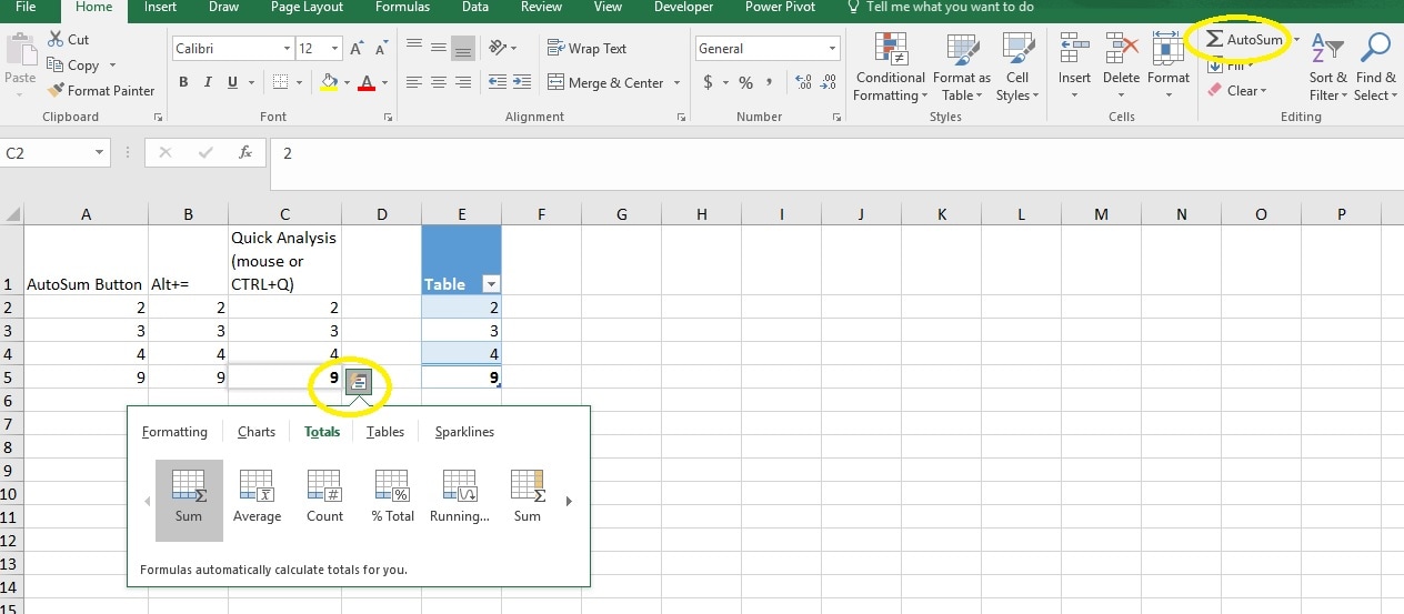
0 Comments
Question: I want to apply conditional formatting to two columns, so that when one column is highlighted by a color, the column next to it is, also.When I am teaching Excel, the question of how to apply conditional formatting to other columns comes up a lot, and in the past I solved it with a macro or an =if rule mimicking conditional formatting, and this is still a good solution. However the clever engineer I am married to showed a me a better, more efficient way, and that is a golden rule: in Excel, efficiency is everything. To start, I am setting up a simple spreadsheet. I have the days of the week in Column A1:A7 and numbers 1-7 in Column B1:B7. For this scenario, I want to say that anything in column B that is greater than 5 is highlighted. Step 1: Make your range a table by pressing CRTL+T at the same time. This inserts a header row, making the table span A1:B8. Step 2: Select your cells that should be affected by the conditional formatting. Step 3: Create a conditional formatting rule. I will use anything above 4 will be highlighted as yellow. a. New Rule b. =$B2>=4 and the formatting is yellow. Using the $B keeps Excel looking in row B to find a value in 4. Step 3: Modify the rules. This will include column A. Go to Modify Rules to open the Conditional Formatting Rules Manager. a. The rules should apply to =$A$2:$B$8. Use F4 to get the magical $ to indicate absolute value. 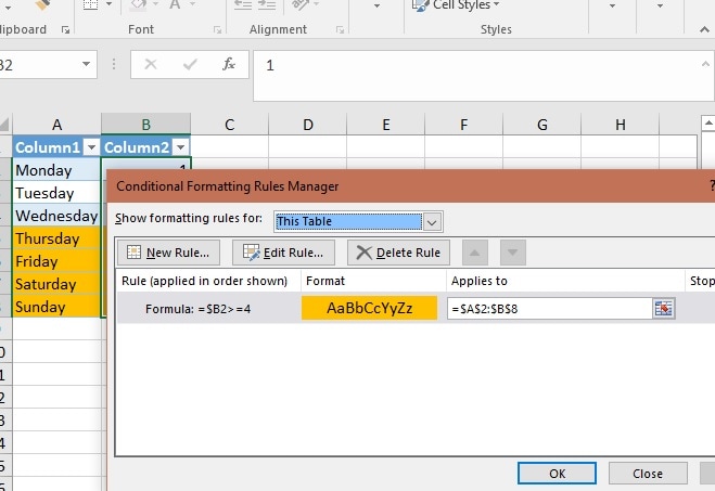 In a class recently, someone asked me how to use Excel for a random drawing. Like all things Excel, it seems like it is possible. Also like all things Excel, it is more complicated than it needs to be. Step One: a. Cell A1: Type Number of Winners b. Cell A2 is the number of winners, and this number can be changed depending on how many prizes are available. In formulas, it is written as $A$2 because it is the only place to look at numbers. 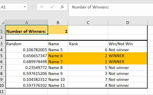 Step Two a. A3 is the =rand() formula This tells excel to create a random number in each cell. If you want random whole numbers, use =randbetween() and choose the numbers you want, such as =randbetween(1,10000) b. B3 is the names of the eligible people. In my example, these names go from B4:B10. c. C3 is a rank formula that is looking at column A and figuring for any cell, how does it relate to the rest of the cells. It is =RANK(A4,$A$4:$A$10) - or whichever rows you use. d. D3 is an if formula that is looking at the number of winners less than or equal to whatever is in A2. =IF(C4<=$A$2,"WINNER","Not winner") e. The conditional formatting is applied to columns B, C, and D. B4 through D10 all have the same conditional formatting, applied one column at a time. This could become a macro because you are doing the same thing three times. f. Go to conditional formatting, new rule, =C4<=$A$2 and pick a color. The C4 is replaced with whatever cell when it is dragged down/across. 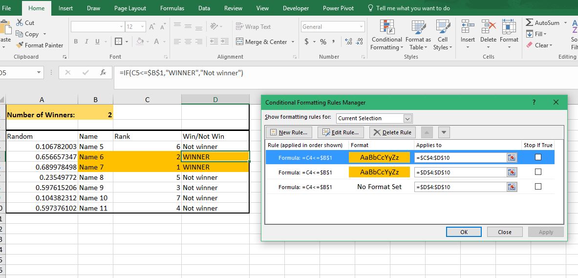 Step Three
The random numbers will always be changing, so copy and paste it either as values with source formatting or (my preference) as a picture so it will be the same every time. Paste it in another area of the sheet, but press the drop down arrow by the paste and choose paste as values and keep the source formatting or paste as picture. This is on a sheet called step 3. If I were doing it, I would paste it on a new sheet as a picture. That way it is frozen in time and you can name the sheet for that week's contest. Paste it in another area of the sheet, but press the drop down arrow by the paste and choose paste as values and keep the source formatting or paste as picture. This is on a sheet called step 3. If I were doing it, I would paste it on a new sheet as a picture. That way it is frozen in time and you can name the sheet for that week's contest. |
AuthorThese are tips and tricks from my Excel adventures. ArchivesCategories
All
|
 RSS Feed