Create a random drawing with Excel

In a class recently, someone asked me how to use Excel for a random drawing.  Like all things Excel, it seems like it is possible.  Also like all things Excel, it is more complicated than it needs to be.

To do this, we use:
=rand
=rank
conditional formatting

Step One:

a. Cell A1: Type Number of Winners
b. Cell A2 is the number of winners, and this number can be changed depending on how many prizes are available.   In formulas, it is written as $A$2 because it is the only place to look at numbers.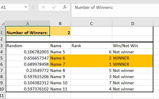

Step Two
a. A3 is the =rand() formula   This tells excel to create a random number in each cell.  If you want random whole numbers, use =randbetween() and choose the numbers you want, such as =randbetween(1,10000)

b. B3 is the names of the eligible people.  In my example, these names go from B4:B10.

c. C3 is a rank formula that is looking at column A and figuring for any cell, how does it relate to the rest of the cells. It is =RANK(A4,$A$4:$A$10)  - or whichever rows you use.

d. D3 is an if formula that is looking at the number of winners less than  or equal to whatever is in A2.   =IF(C4<=$A$2,"WINNER","Not winner")

e. The conditional formatting is applied to columns B, C, and D. B4 through D10 all have the same conditional formatting, applied one column at a time.  This could become a macro because you are doing the same thing three times.

f.  Go to conditional formatting, new rule,  =C4<=$A$2   and pick a color.  The C4 is replaced with whatever cell when it is dragged down/across.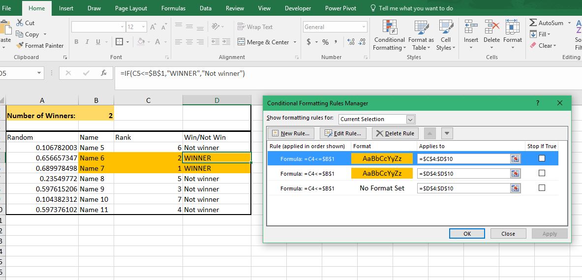  

Step Three

The random numbers will always be changing, so copy and paste it either as values with source formatting or (my preference) as a picture so it will be the same every time.

Paste it in another area of the sheet, but press the drop down arrow by the paste and choose paste as values and keep the source formatting or paste as picture.  This is on a sheet called step 3.

If I were doing it, I would paste it on a new sheet as a picture.  That way it is frozen in time and you can name the sheet for that week's contest.
Paste it in another area of the sheet, but press the drop down arrow by the paste and choose paste as values and keep the source formatting or paste as picture.  This is on a sheet called step 3.

If I were doing it, I would paste it on a new sheet as a picture.  That way it is frozen in time and you can name the sheet for that week's contest.